Visualising data in Python: Plotly vs Matplotlib

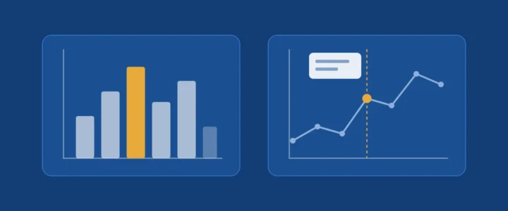
« Which library should I use? » is the question almost every student asks when discovering data visualisation in Python. The right answer is not a name but another question: where will your chart be read? On a printed page, in a thesis, in a dashboard shared with management? Matplotlib and Plotly serve different needs because they rest on different ideas of what a figure is.

Learning objectives

• distinguish a static figure (an image) from an interactive one (a program running in the browser);
• understand Matplotlib backends and the difference between raster and vector formats;
• produce the same chart with both libraries and export it correctly;
• choose the right tool for a given communication situation.

1. Two ideas of a figure

1.1 Matplotlib: drawing an image

Matplotlib, the long-standing library of the scientific Python ecosystem, draws. The end result is an image, produced by a rendering engine called a backend. The documentation distinguishes two families:

• interactive backends, which display the figure in a window (Qt, Tkinter, macOS);
• non-interactive backends, which write a file: Agg for raster images (PNG), and vector backends for PDF, SVG and PS/EPS.

The raster / vector distinction is essential for academic documents. A raster image is a grid of pixels: enlarged, it blurs. A vector image describes geometric shapes: it stays sharp at any size and its text remains selectable. For a paper or a thesis, prefer PDF or SVG.

1.2 Plotly: describing a figure, letting the browser render it

Plotly works differently. In Python, you build a description of the figure (a data structure listing traces, axes and legends). That description is then rendered by the plotly.js JavaScript library in a browser. Hence built-in interactivity: zoom, hover tooltips, hiding a series with a click on the legend.

2. Worked example: the same chart, twice

Take the number of entrance exam candidates over five sessions (fictitious figures, for illustration only).

2.1 With Matplotlib (object-oriented interface)

import matplotlib.pyplot as plt

years = [2022, 2023, 2024, 2025, 2026]
candidates = [412, 538, 601, 744, 820]

fig, ax = plt.subplots(figsize=(6, 3.5))
ax.plot(years, candidates, marker="o")
ax.set_title("Entrance exam candidates")
ax.set_xlabel("Session")
ax.set_ylabel("Number of candidates")
ax.set_xticks(years)
ax.grid(alpha=0.3)

fig.savefig("candidates.pdf")              # vector, for the thesis
fig.savefig("candidates.png", dpi=200)     # raster, for a slide

Note two habits worth adopting. First, the object-oriented interface (fig, ax = plt.subplots()) rather than global plt.plot() calls: you always know which chart you are acting on, which becomes essential as soon as a figure has several panels. Second, savefig infers the format from the file extension; the dpi parameter sets the resolution of raster images.

2.2 With Plotly Express

import plotly.express as px

fig = px.line(
    x=[2022, 2023, 2024, 2025, 2026],
    y=[412, 538, 601, 744, 820],
    markers=True,
    labels={"x": "Session", "y": "Number of candidates"},
    title="Entrance exam candidates",
)

fig.write_html("candidates.html", include_plotlyjs="cdn")  # interactive
fig.write_image("candidates.svg")                           # static

Two exports, two uses. write_html produces a self-contained page; the include_plotlyjs option decides whether the JavaScript library is embedded in the file (heavy, but readable offline) or loaded from a CDN (light, but requires internet access). write_image produces a static image in PNG, JPEG, WebP, SVG or PDF; it requires the Kaleido package (version 1.0.0 or later according to Plotly’s current documentation).

3. Decision table

Situation	Recommended choice	Why
Figure for a paper, thesis or dissertation	Matplotlib	Fine typographic control and vector PDF or SVG export
Shared dashboard, reader-driven exploration	Plotly	Zoom, tooltips and filters with no extra code
Very large number of points	Matplotlib	An image stays light; an interactive chart must ship all the data to the browser
HTML report sent to management	Plotly	A single file, readable in any browser
Lecture slide	Either	High-resolution PNG from Matplotlib, or a static image exported from Plotly

4. Beyond the tool: the rules of a good chart

Whatever the library, a teaching chart follows a few simple rules:

• a title that states what to see, not just what is measured: « Applications doubled in five years » rather than « Applications »;
• labelled axes with units;
• colours readable by everyone, including colour-blind readers, and never colour as the only carrier of information;
• no gratuitous effects: decorative 3D and shadows distort how values are read.

Common mistakes

• Pasting a blurry screenshot of a chart into a thesis instead of a vector export.
• Mixing global plt. calls and ax objects in the same figure.
• Sending a CDN-based Plotly HTML file to a reader who will open it offline.
• Choosing interactivity on principle when the reader will print the report.

Key takeaway

Matplotlib produces images to be read; Plotly produces applications to be explored. Choose according to where the chart will be read, then craft its message, which matters more than the tool.

References

• Matplotlib, Backends.
• Plotly, Static image export in Python.
• Plotly, Interactive HTML export in Python.